Data Management Workflow for Bioinformatics & Imaging Projects#
This document summarizes best practices for multi-level data management in a research laboratory (e.g., CNRS/INSERM/University labs), with a focus on imaging and bioinformatics workflows. It is designed for PhD students, postdocs, and engineers who need a clear overview of how to store, process, and archive research data.
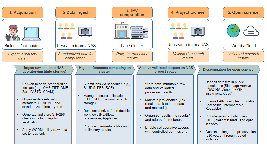
Levels of Storage#
Research data circulates across several infrastructure layers:
Acquisition workstation (microscope/sequencer computer)
Temporary buffer only (local disk of the instrument PC).
Data generated in proprietary formats (e.g.,
.czi,.lif,.nd2,.fast5).Action: transfer as soon as possible to institutional storage.
Laboratory/Institute NAS (Network Attached Storage)
Central project space for the team.
Stores raw immutable data (
raw/) and validated results (results/,release/).Snapshots, quotas, and backups are usually managed by the IT team.
Best practice: enforce WORM policy (write once, read many) on raw data.
University / Regional HPC cluster
Provides CPUs, GPUs, and large temporary scratch storage.
Used for heavy computation (segmentation, alignment, assembly, deep learning).
Scratch is temporary (30–60 days auto-purge).
Results must be copied back to NAS.
National infrastructures (CNRS/INSERM/GENCI/IDRIS/CC-IN2P3)
Large-scale storage and GPU/CPU compute for very heavy projects.
Access requires project allocation.
Used for multi-terabyte/petabyte datasets.
Archival & Open Science repositories
Cold storage (LTO tape, S3 Glacier) for long-term preservation (≥10 years).
Public archives for dissemination:
Imaging: BioImage Archive
Sequencing: ENA / SRA / EGA
Processed data, scripts: Zenodo, OSF, institutional repositories
Ensures compliance with FAIR principles.
Data Lifecycle Example (Cell Segmentation with U-Net)#
Step 1 — Acquisition
Confocal images acquired in
.cziformat (~400 GB dataset).
Step 2 — Ingest to NAS
Convert to OME-TIFF/OME-Zarr.
Generate
MANIFEST.sha256checksums.Store in
/data/projects/PRJ-XXXX/raw/.Apply read-only permissions (WORM).
Step 3 — HPC Computation
Transfer dataset to cluster scratch with
rsyncorGlobus.Submit deep learning job (U-Net segmentation) via SLURM.
Produce masks (OME-TIFF, compressed) + measurement tables (CSV).
Step 4 — Archive to NAS
Store results in
/results/segmentation/(masks, tables, QC reports).Purge intermediate files.
Add README with workflow version, model, GPU used.
Step 5 — Dissemination
Deposit representative images + masks in BioImage Archive.
Publish tables + scripts in Zenodo with DOI.
Keep complete raw dataset in cold archive (tape/Glacier).
Integrity & Security#
Checksums:
# Generate manifest
find raw -type f -print0 | xargs -0 sha256sum > MANIFEST.sha256

# Verify later
sha256sum -c MANIFEST.sha256 | tee verify_$(date +%F).log
WORM policy:#
POSIX: chmod -R a-w raw/
Linux: chattr +i file
ZFS: snapshots + holds
S3/Ceph: Object Lock (compliance mode)
Backup (3-2-1 rule):
3 copies (production, local backup, off-site backup)
2 types of media (disk + tape)
1 copy offline/off-site
Key Takeaways#
Cluster scratch is temporary → always copy validated results back to NAS.
NAS is the project reference → raw data immutable, results organized and documented.
Public archives ensure FAIRness → publish representative datasets with DOI.
Cold storage ensures longevity → keep full raw + release packages for ≥10 years.
Engineer’s role → manage transfers, integrity, policies, documentation, and training.